Weak Gravitational Lensing of the Cosmic Microwave Background
Yuuki Omori (U.Chicago/KICP)
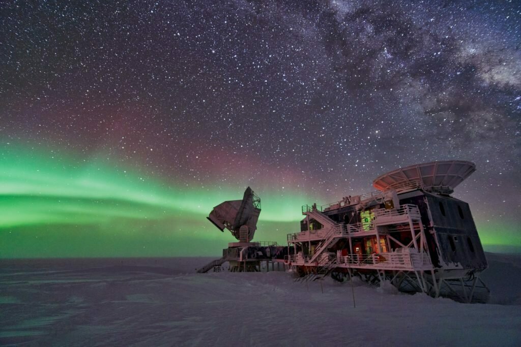
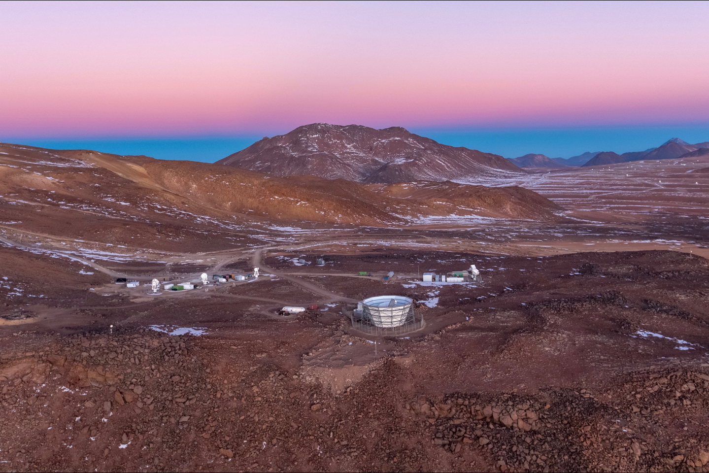
Credit: Aman Chokshi (2021 Winter Over)


Cosmic history
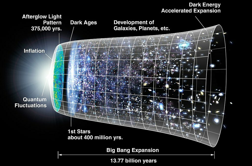
1
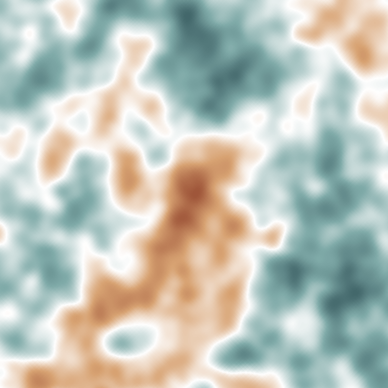
Cosmic microwave background
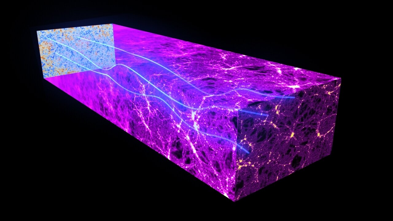
CMB
(source z~1100)
2
CMB weak lensing
CMB
(source z~1100)
2
signal peak
z~2
Source galaxies
CMB weak lensing
CMB
(source z~1100)
2
signal peak
z~2
Source galaxies
signal peak
z~0.5
CMB weak lensing
2
CMB
(source z~1100)
signal peak
z~2
Source galaxies
signal peak
z~0.5
CMB weak lensing
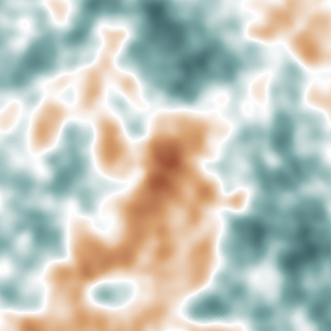
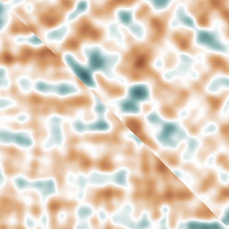
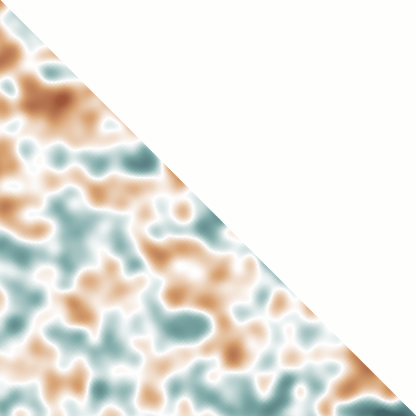
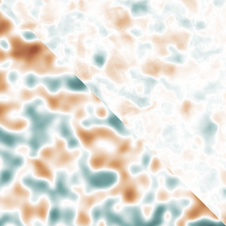
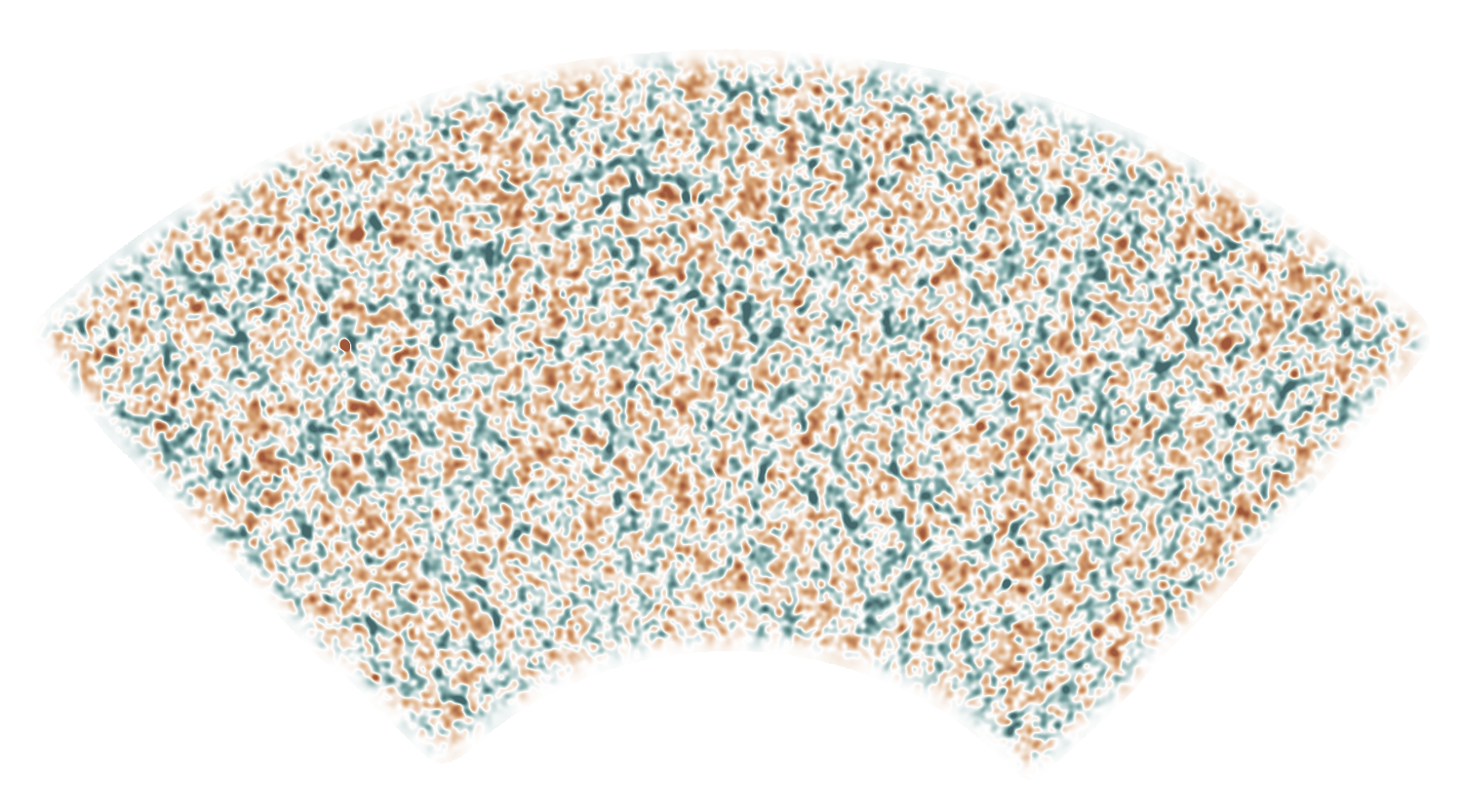
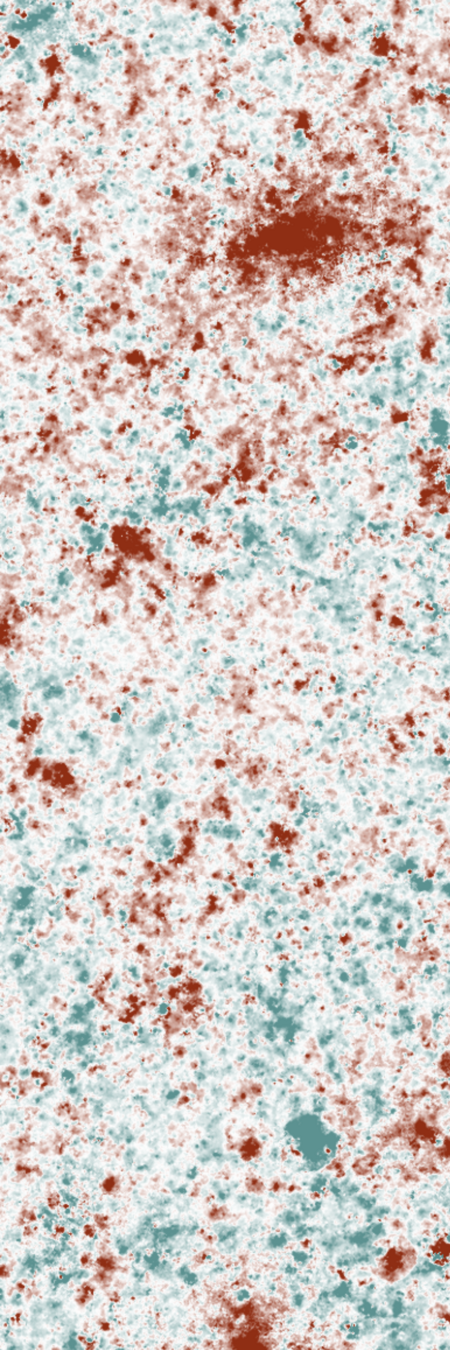
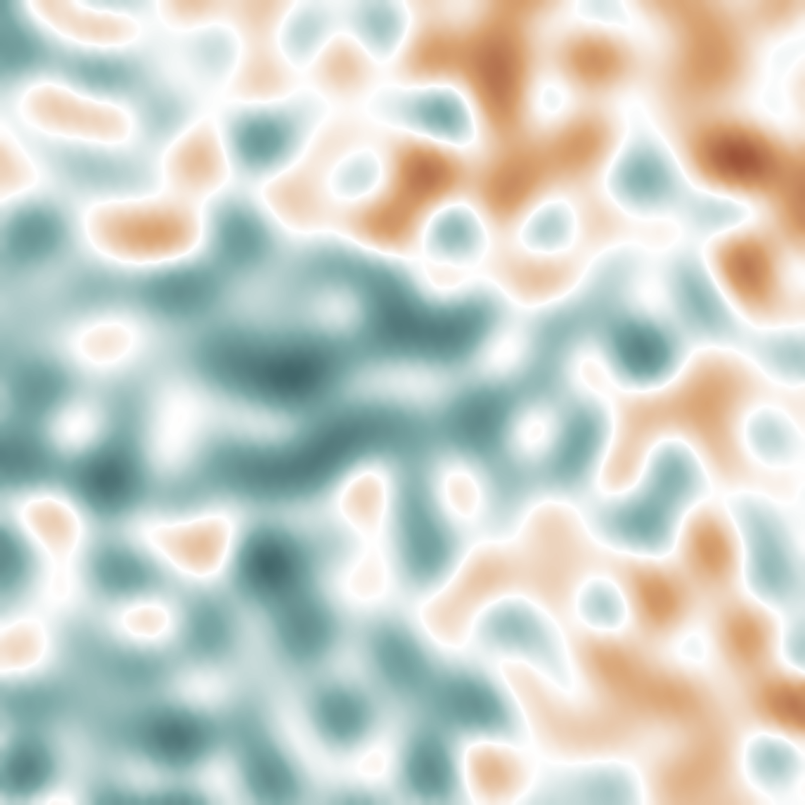
Undistorted temperature map
3
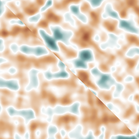
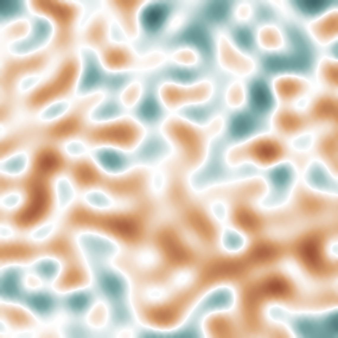
CMB weak lensing
Distorted temperature map
T
Undistorted temperature map
3
CMB weak lensing
Distorted temperature map
Undistorted stokes Q/U map
Distorted stokes Q/U map
T
Q
U
Undistorted temperature map
3
CMB weak lensing
Distorted temperature map
Undistorted E/B map
Distorted E/B map
T
E
B
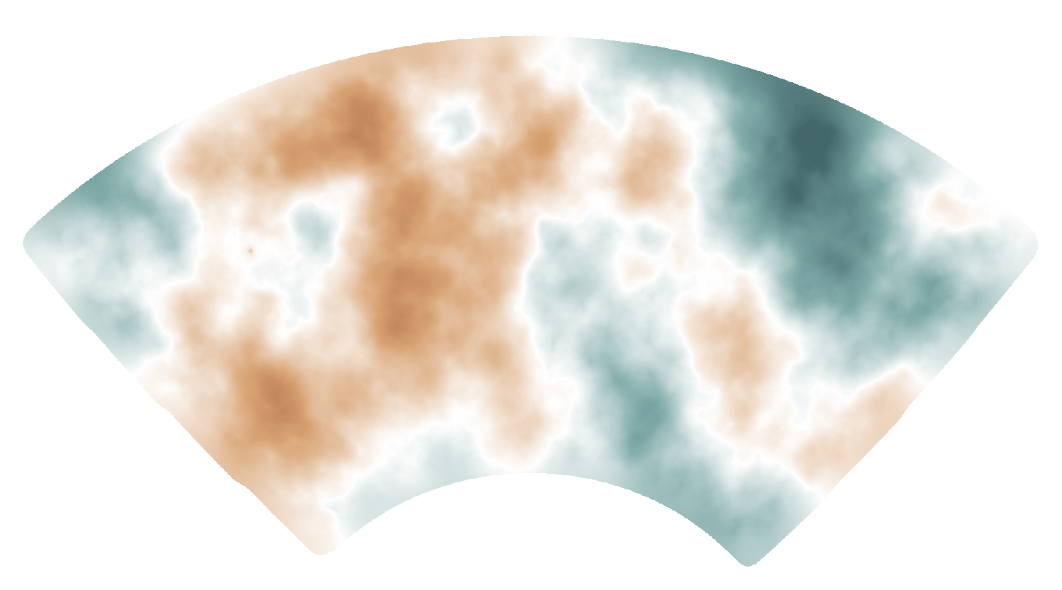
Lensing reconstruction
3D gravitational potential
4
3D gravitational potential
2D potential
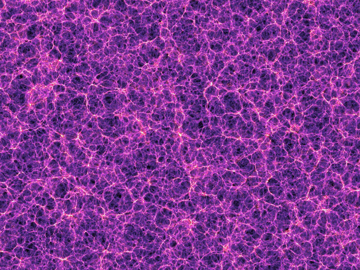
4
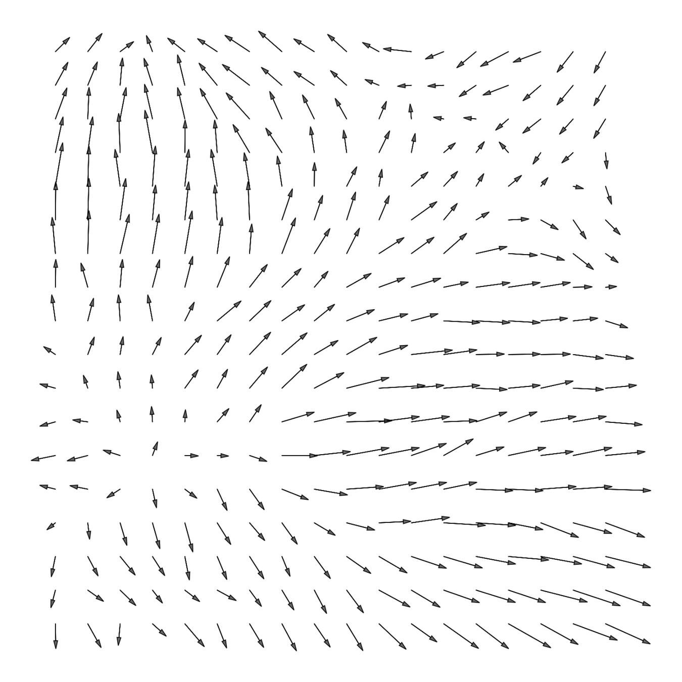
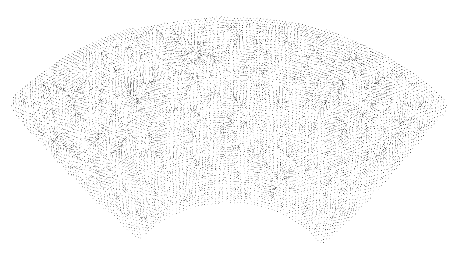
Lensing reconstruction
3D gravitational potential
2D potential
Deflection
4
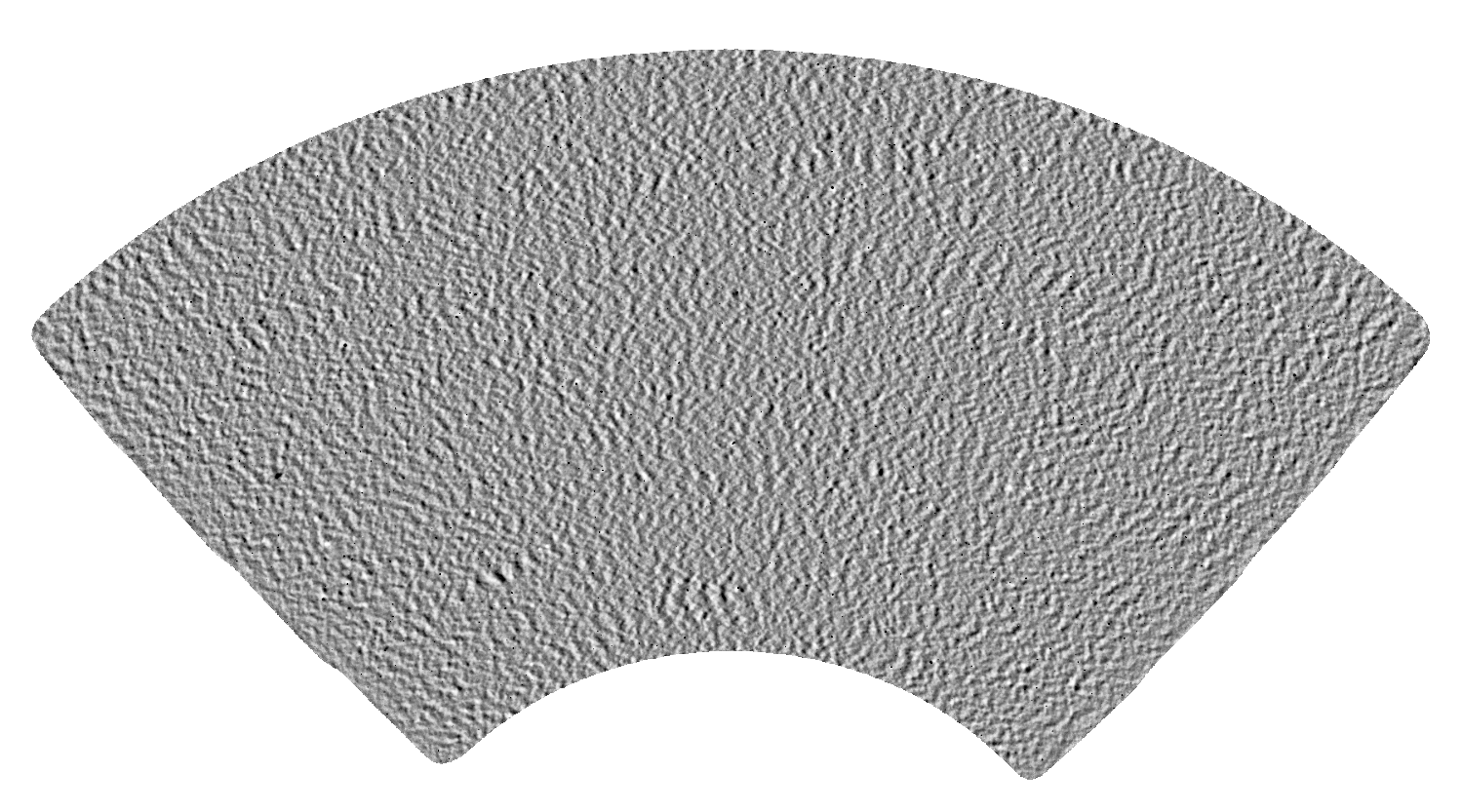
Convergence
Lensing reconstruction
Two independent modes become correlated through the lensing potential
5
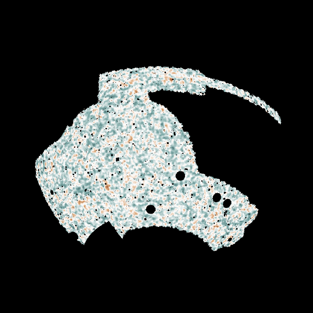
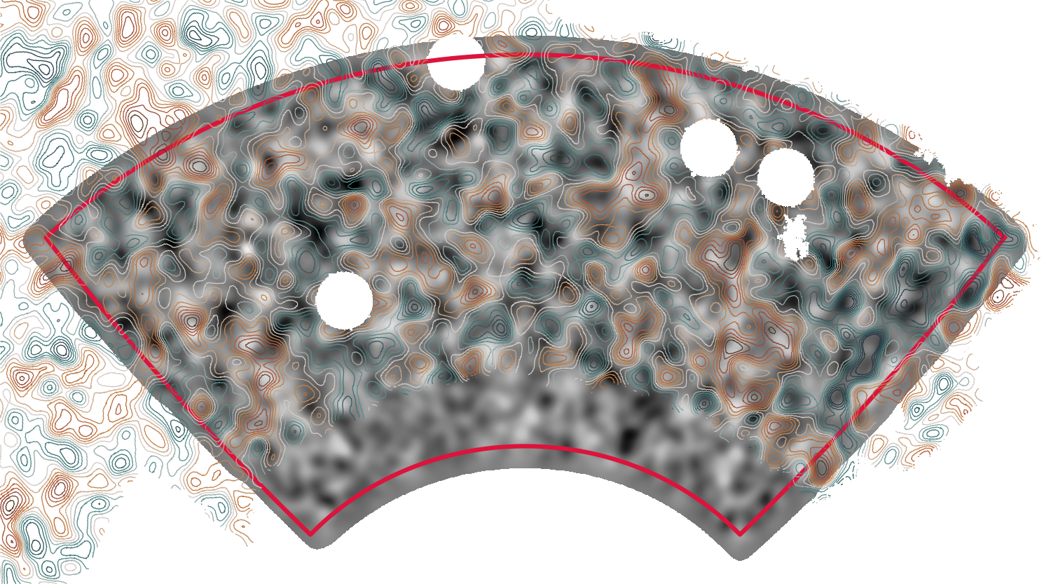
Lensing reconstruction
SPT-3G lensing map
(see also: Omori+ 2017, Omori+ 2023)
6
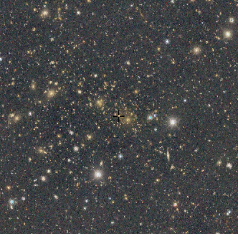
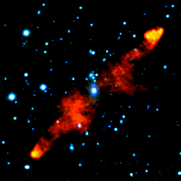
Foregrounds (temperature)
7
SPT-3G temperature map
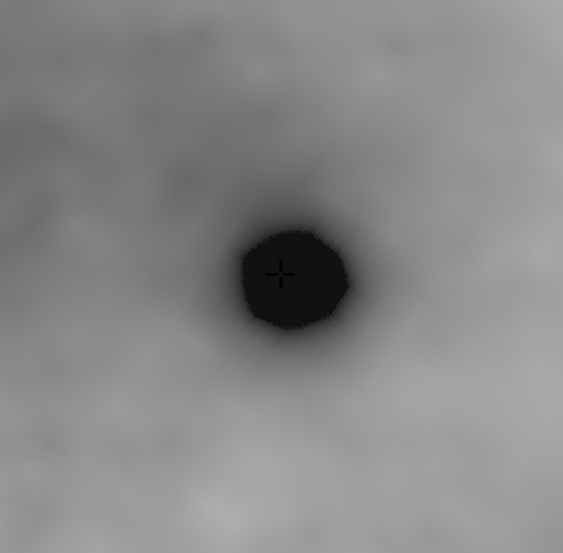
SPT-3G temperature map
SPT-CLJ0234-5831
7
Foregrounds (temperature)
SPT-3G temperature map
SPT-CLJ0234-5831
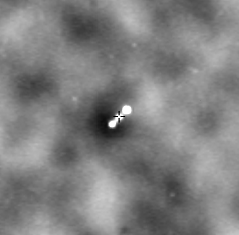
7
Foregrounds (temperature)
SPT-3G temperature map
PKS 2356-61
SPT-CLJ0234-5831
7
Foregrounds (temperature)
8
Mitigation strategies for temperature biases
- Vary input .
- Use deprojection techniques
- (Madhavacheril&Hill2018, Raghunathan& Omori2023).
- (Madhavacheril&Hill2018, Raghunathan& Omori2023).
- Use hardening techniques (point-source/profile hardening).
- Use shear-based lensing estimator (Schaan & Ferraro 2019).
- Use the combinations of above.
Agora simulation (Omori 2022)
Multi-Dark Planck 2
N-body simulation
(Klypin+ 2017)


9
tSZ
kSZ
CIB
radio
Foregrounds (temperature)
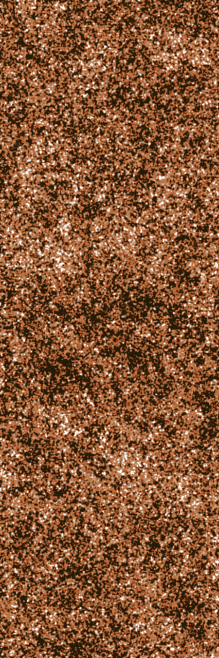
10
Polarization

T
Galaxy cluster
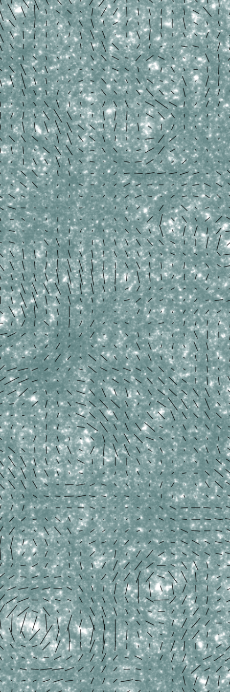
10
Polarization
- Fewer astronomical sources are polarized (less prone to astrophysical systematic biases)
Galaxy cluster
T
Q
U

Point source
11
Polarization
- Fewer astronomical sources are polarized (less prone to astrophysical systematic biases)
- Less affected by atmospheric noise (lower 1/f noise)

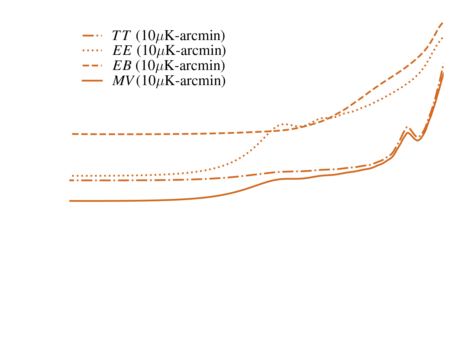
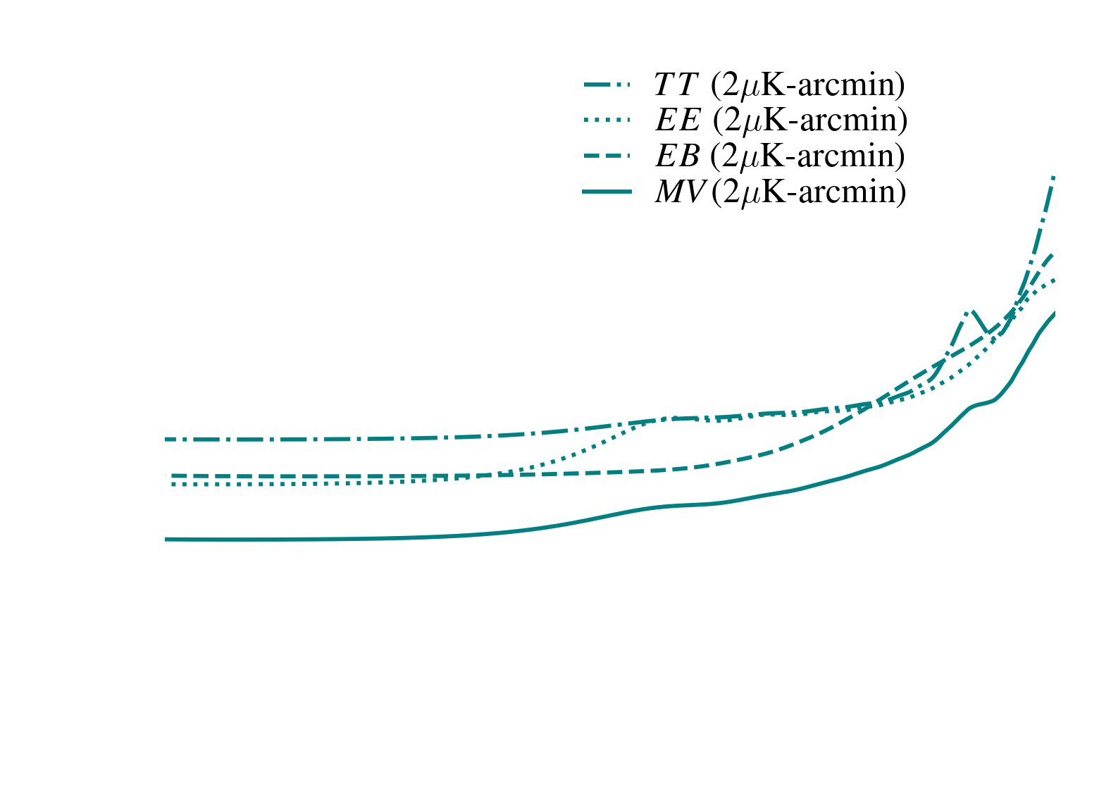
12
Polarization
- Instrumental noise in polarization is higher (and lensing reconstruction scales as noise )
- The survey needs to be sufficiently deep to fully take advantage of polarization
2
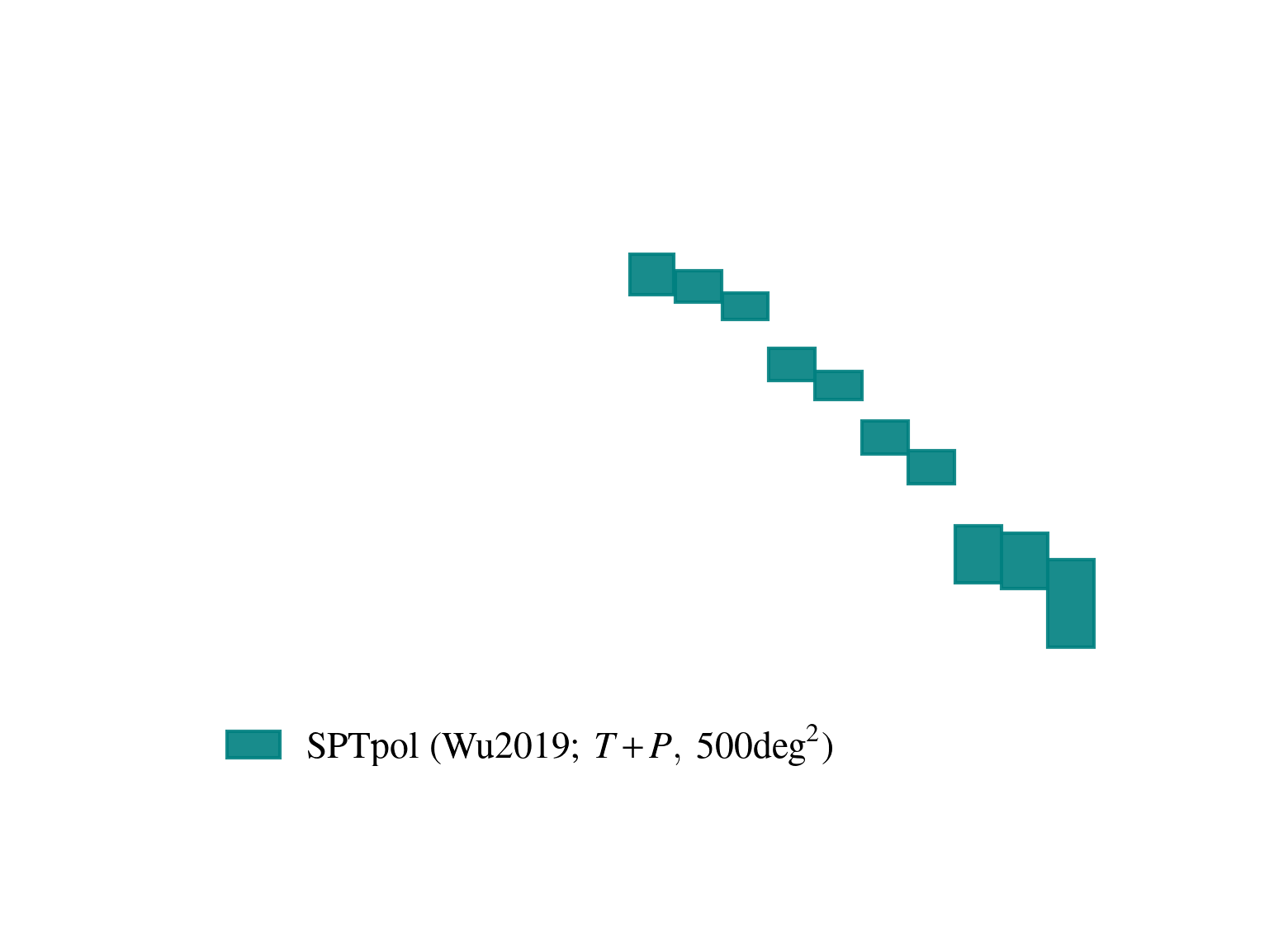
14
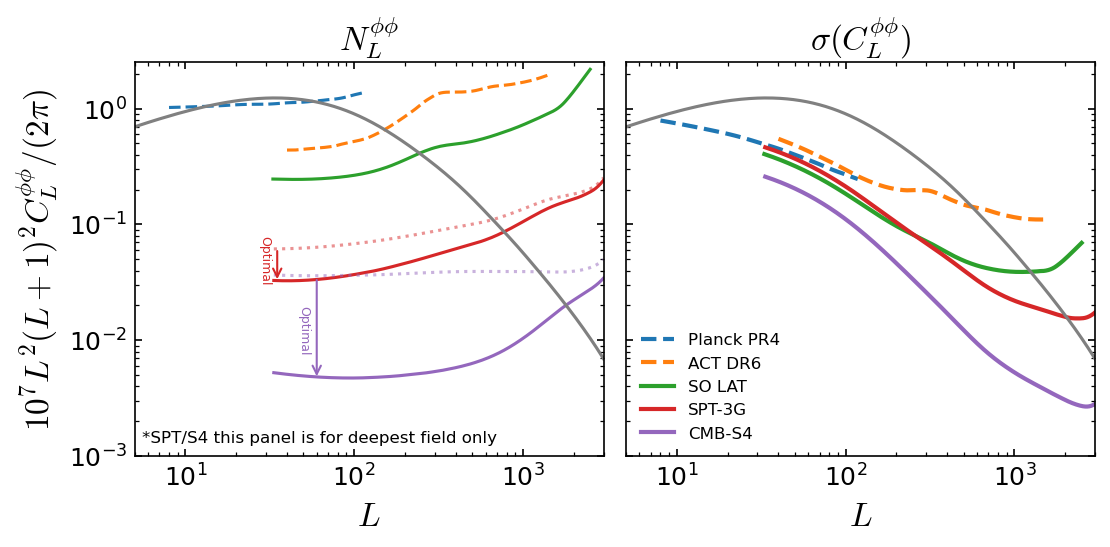
Lensing noise comparison
Text
Experiment 1:
Experiment 2:
SPT-3G -> P dominated
SimonsObs -> non-negligible contribution from T
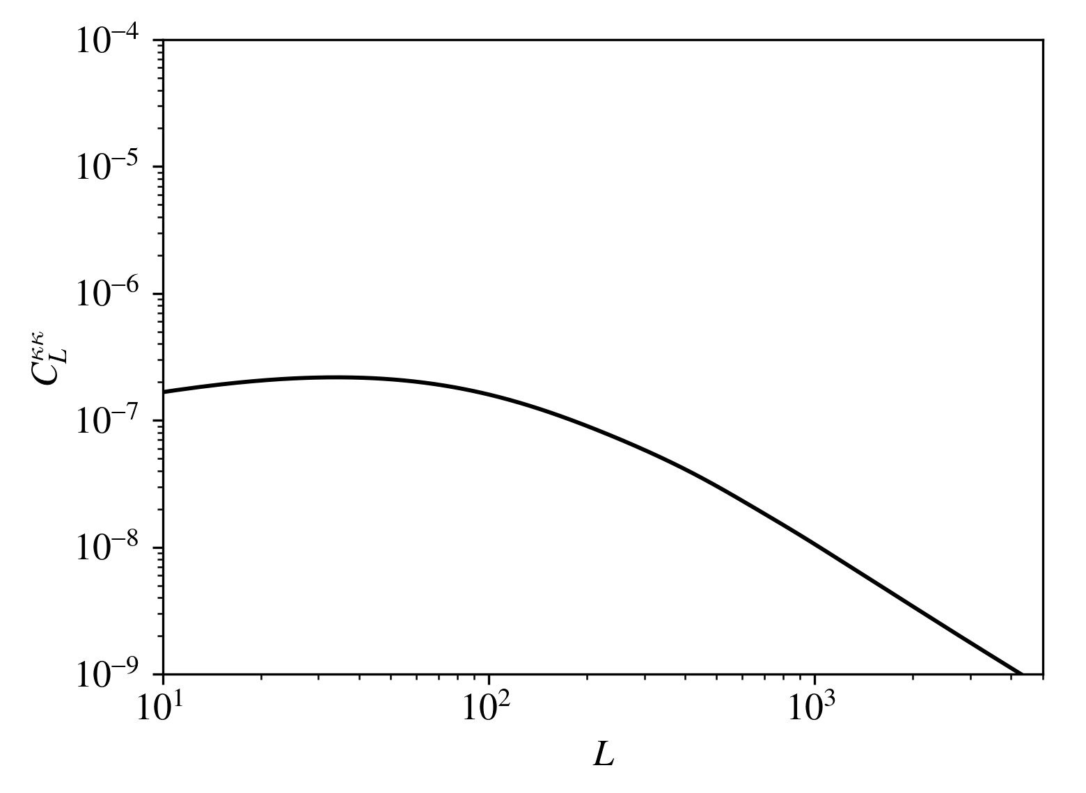
Baryons?
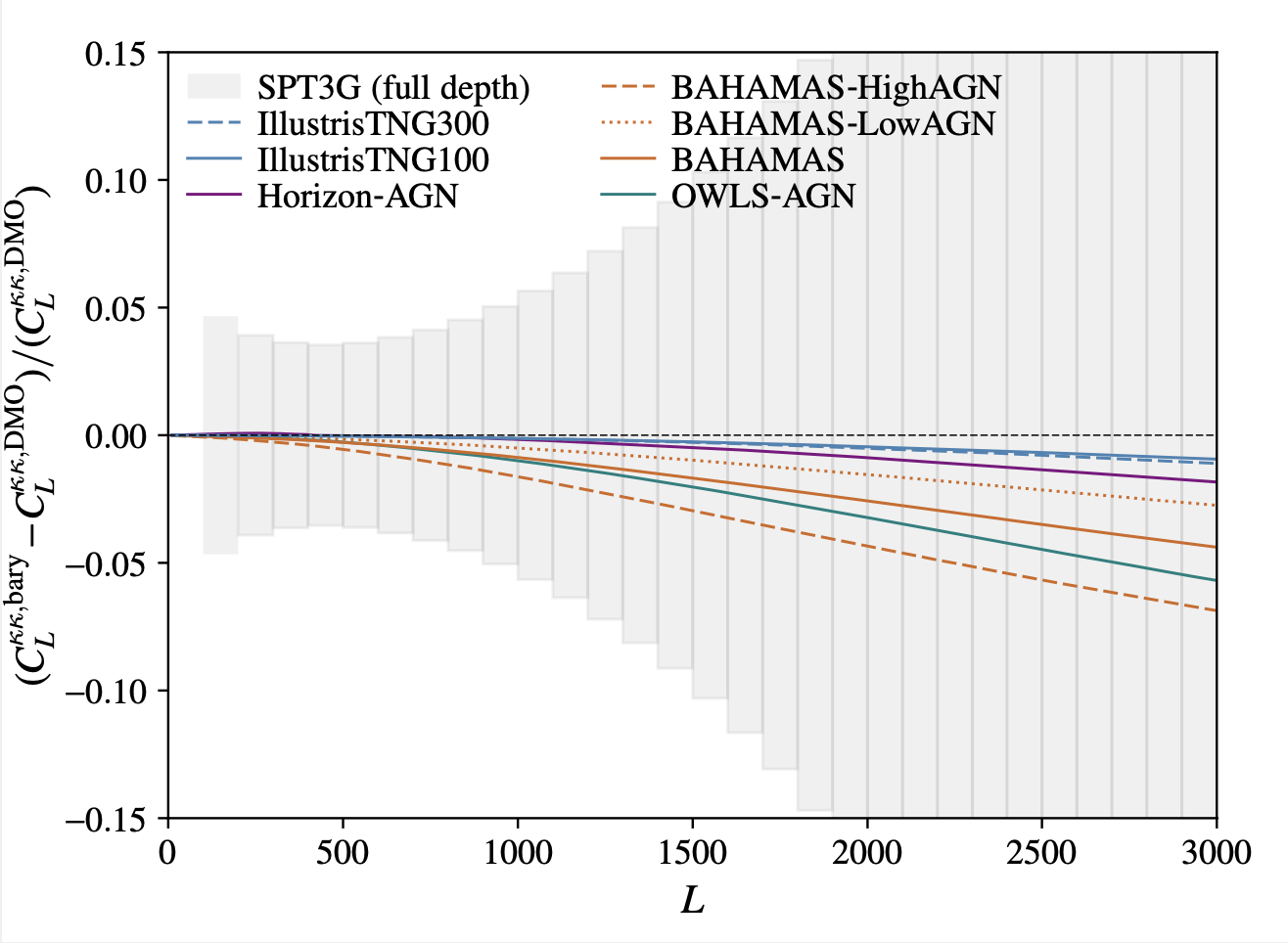
- For CMB lensing auto-spectrum, the impact of Baryons is small (signal peaks at z~2)
- For cross-correlations, the impact depends on the redshift of the other tracer.
15
Current state of CMB lensing
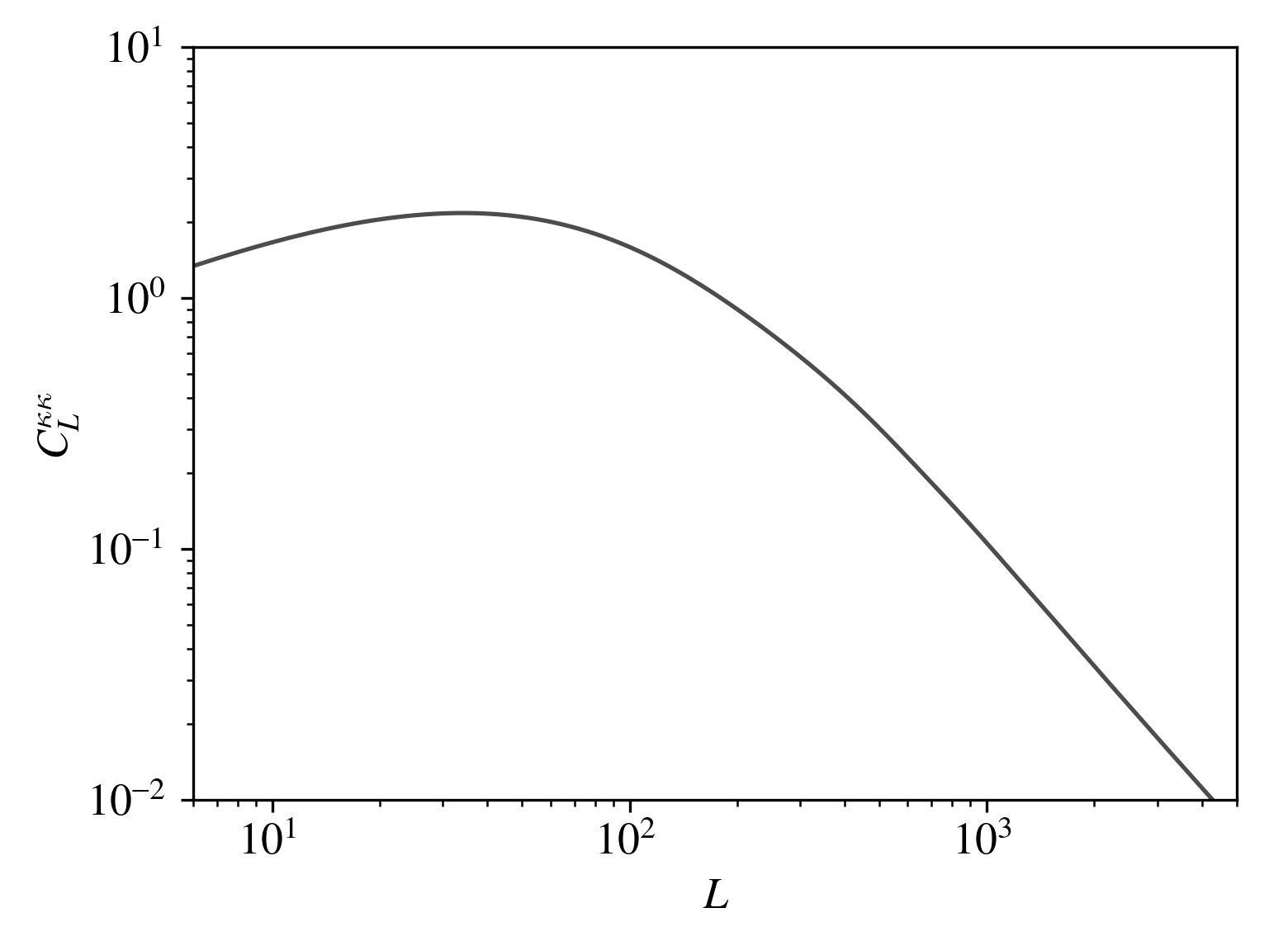
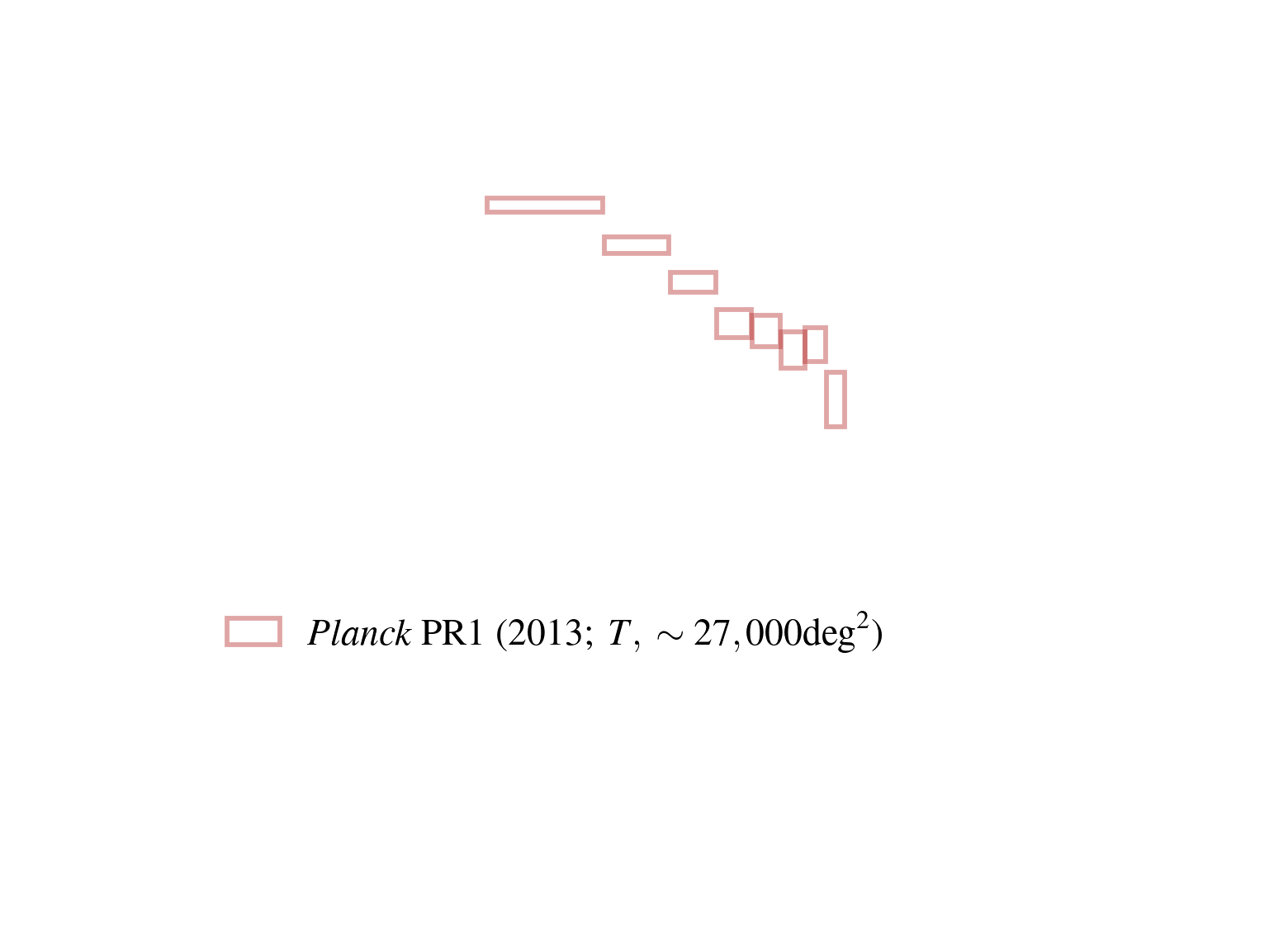
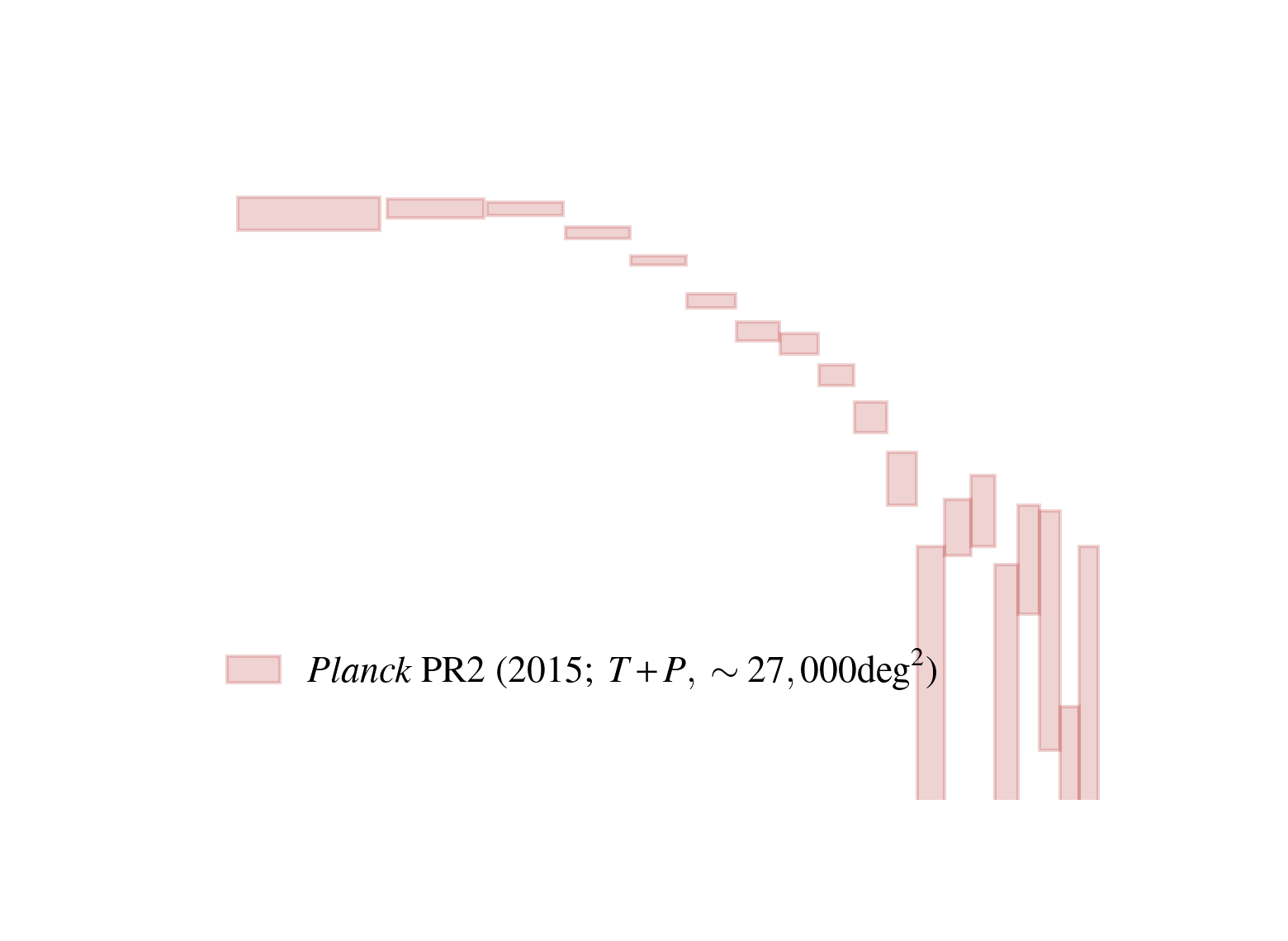
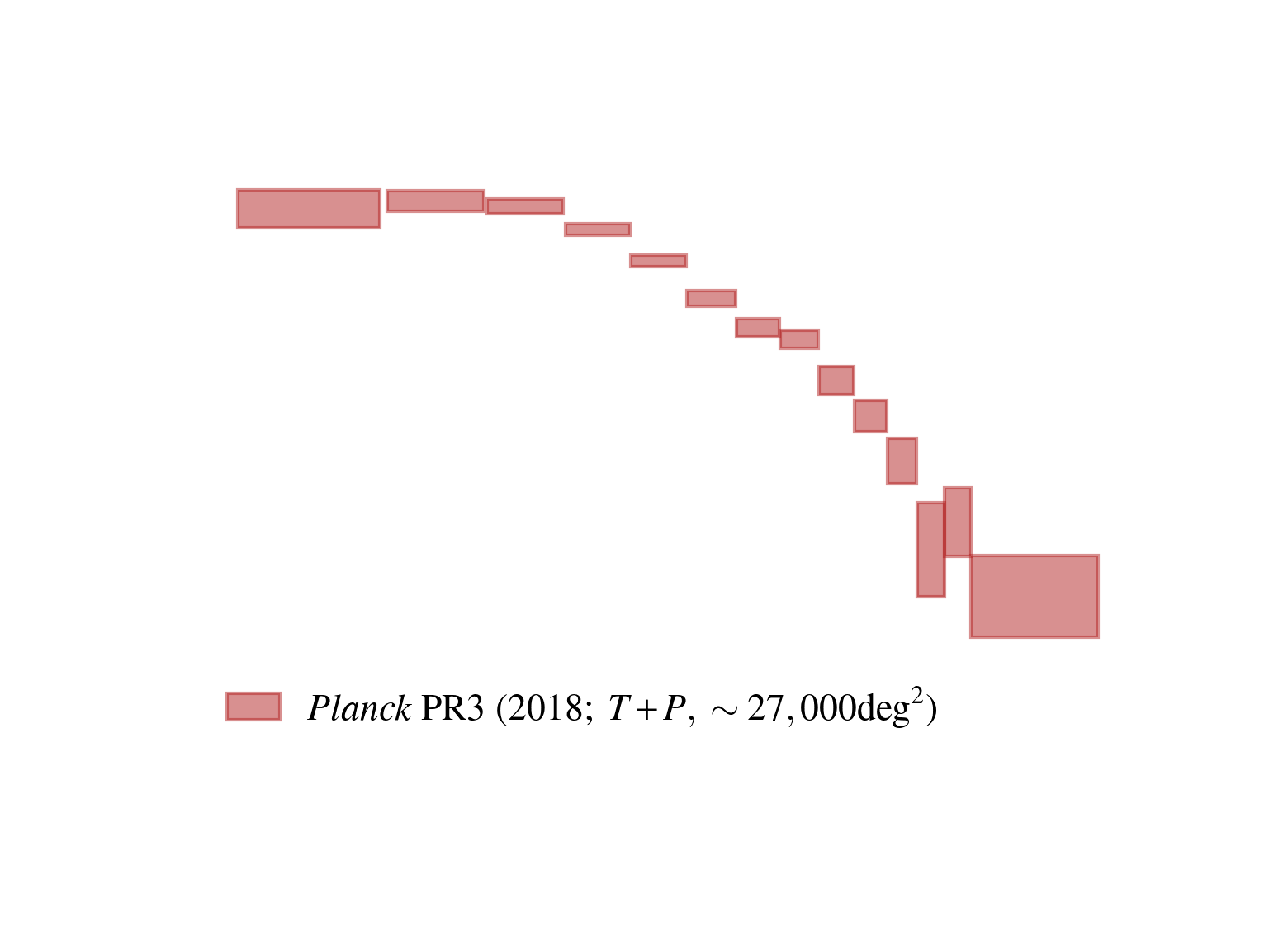
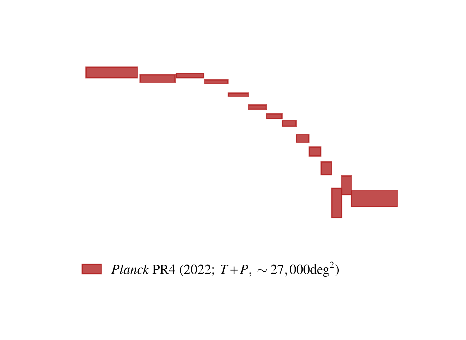
Planck
16
Current state of CMB lensing
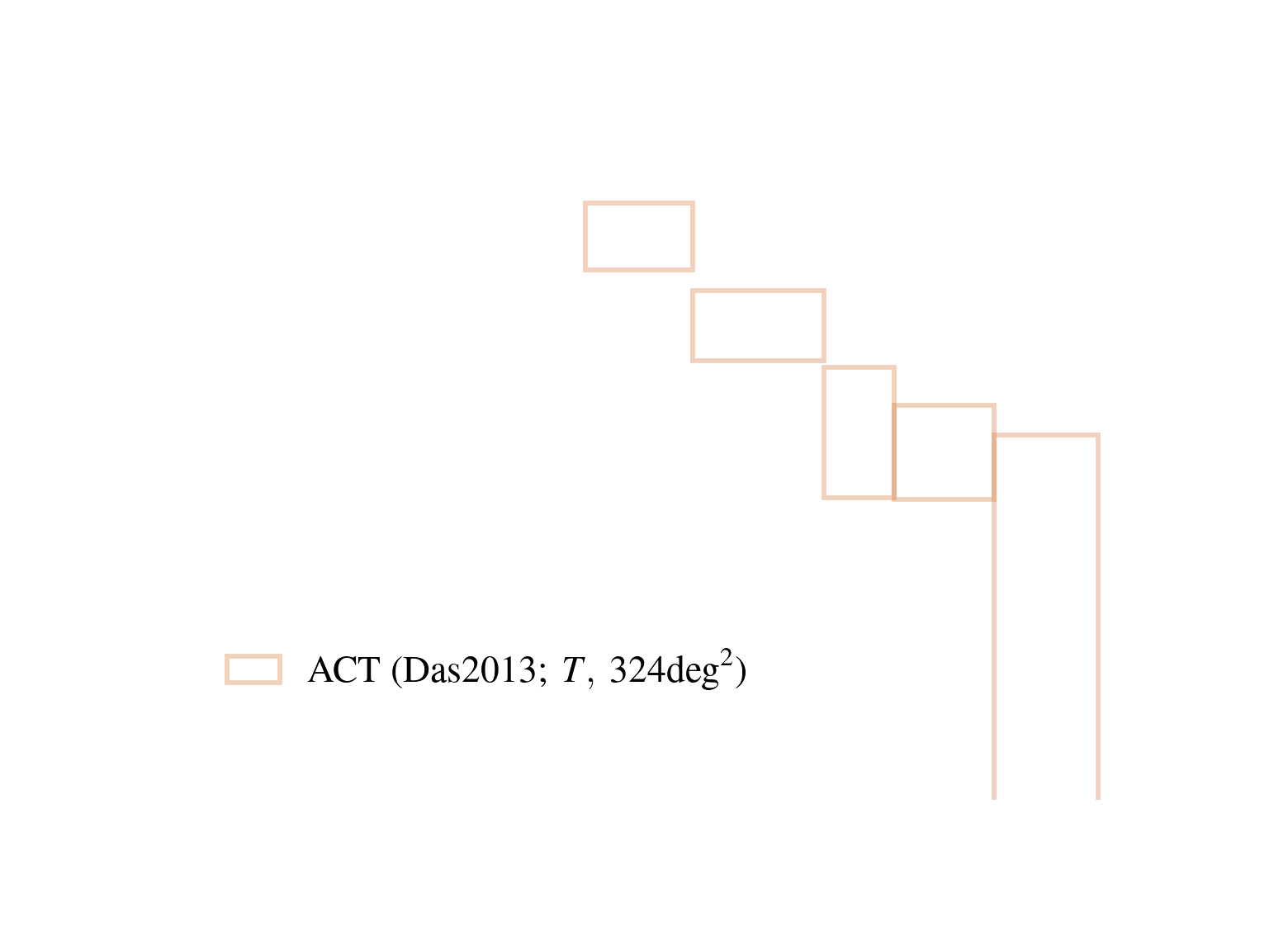
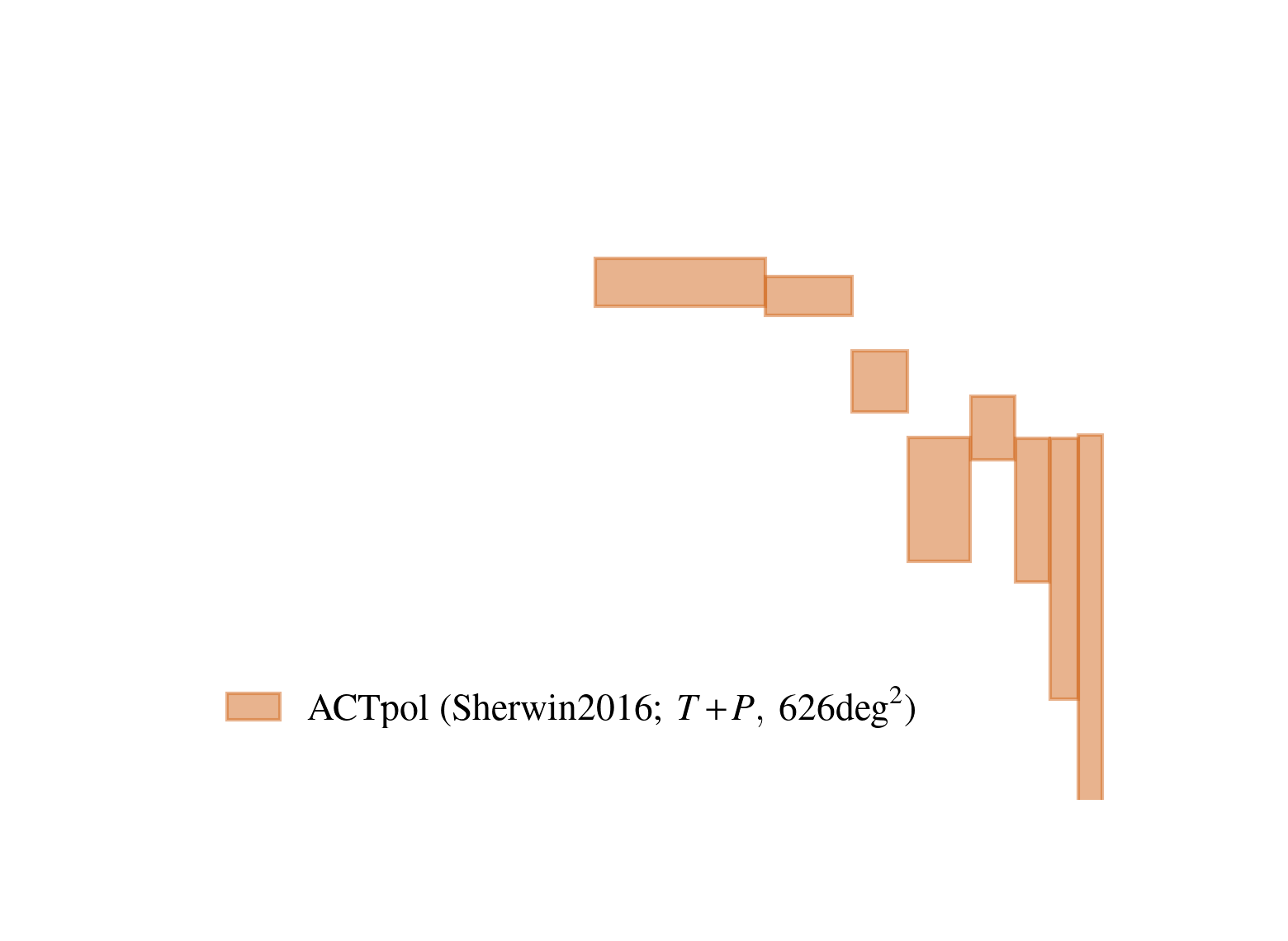
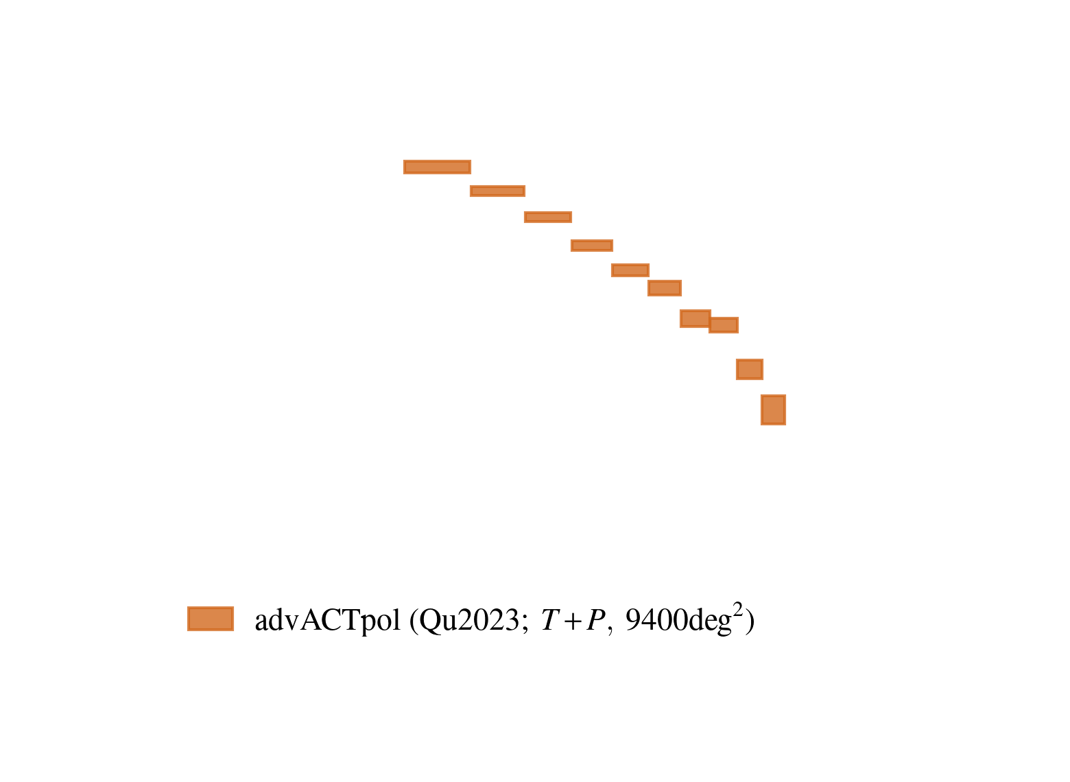
Atacama Cosmology Telescope
17
Current state of CMB lensing
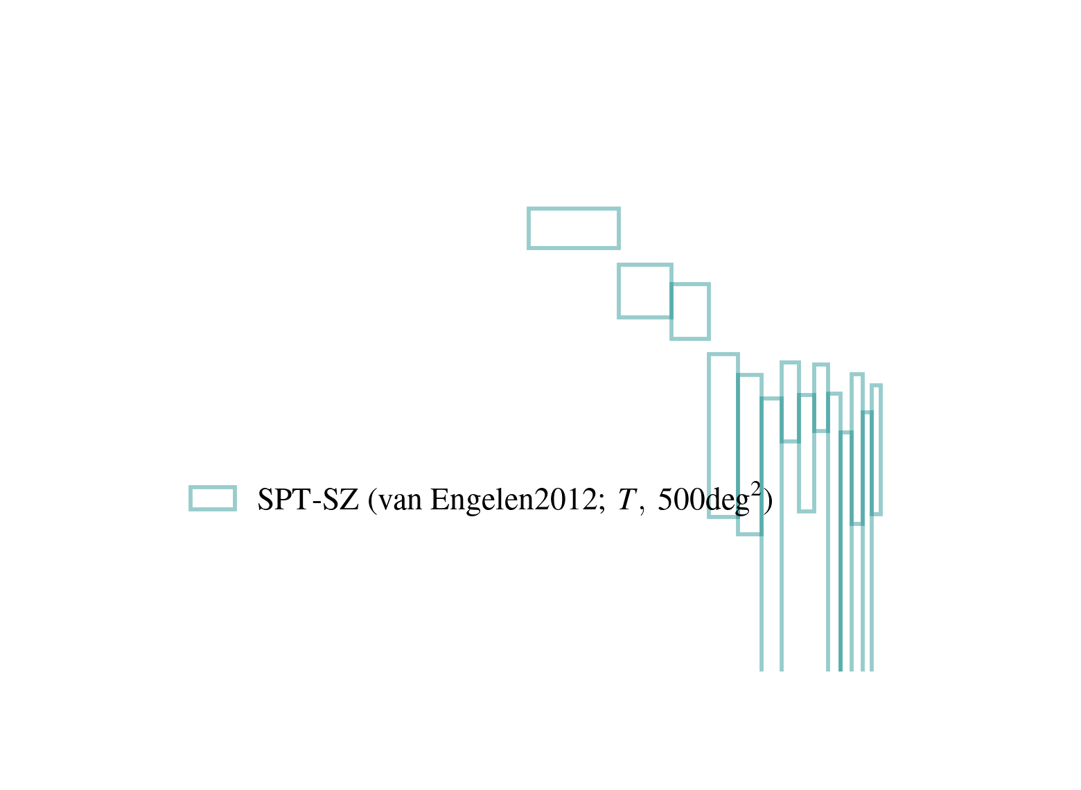
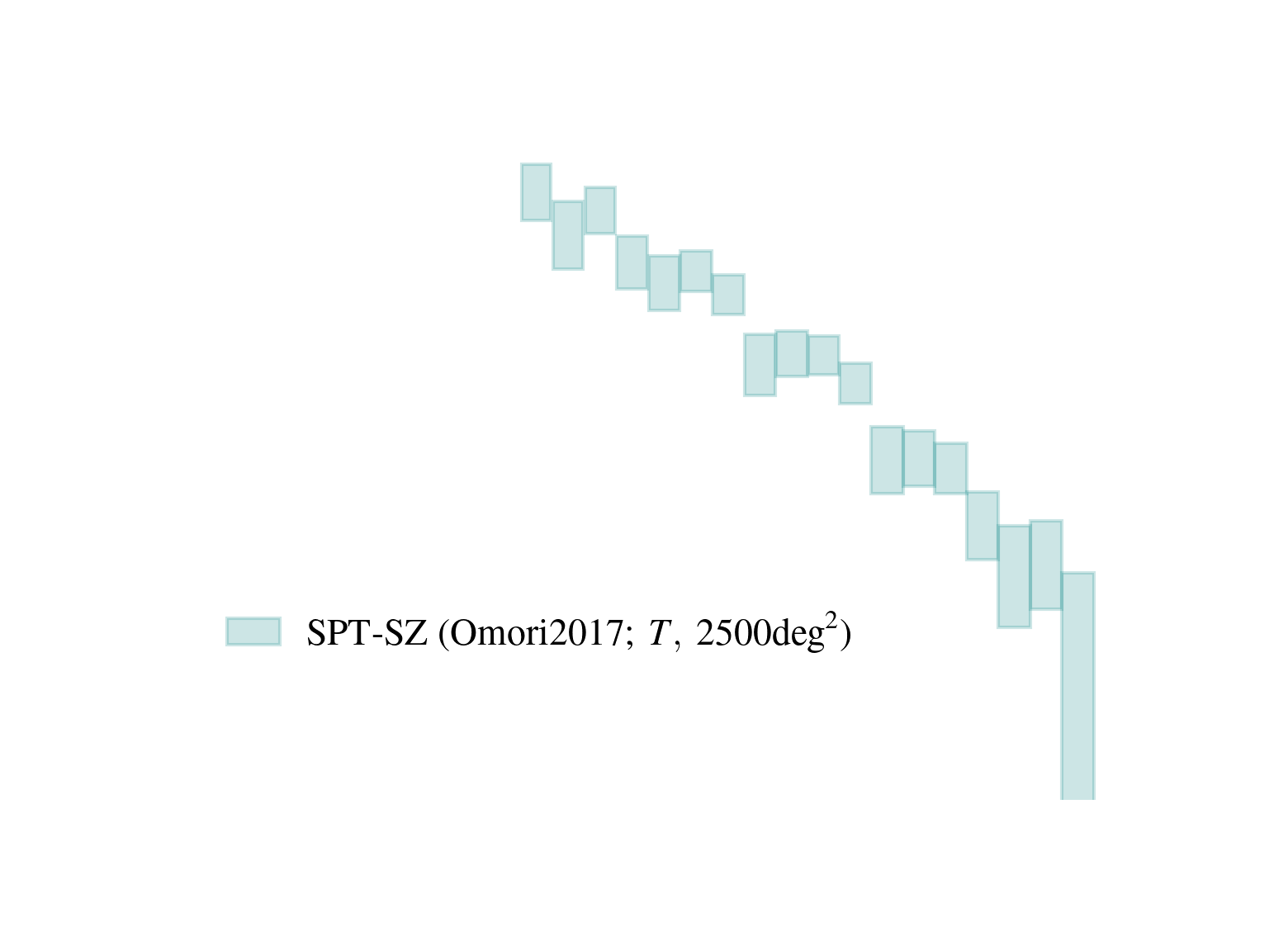
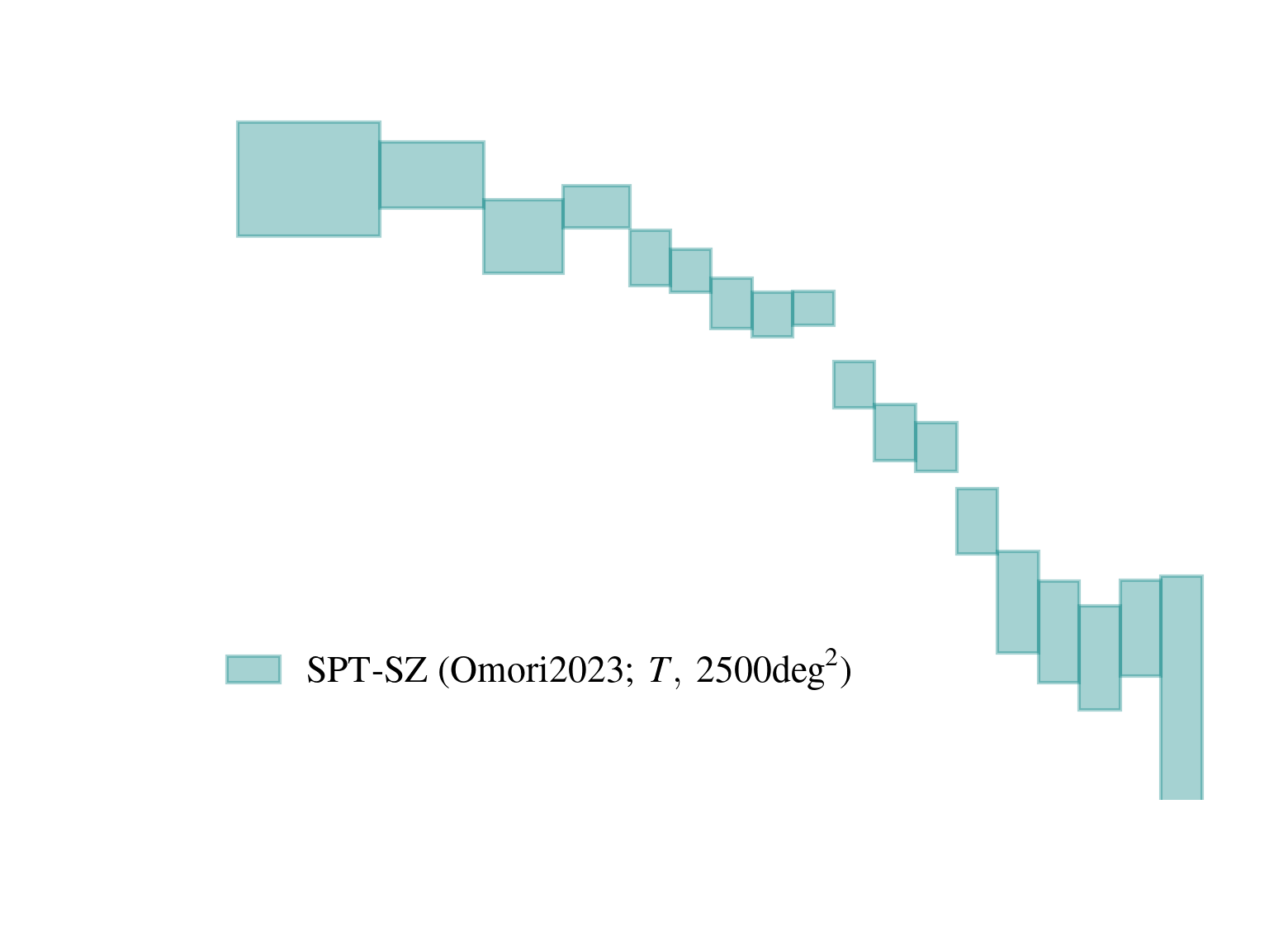
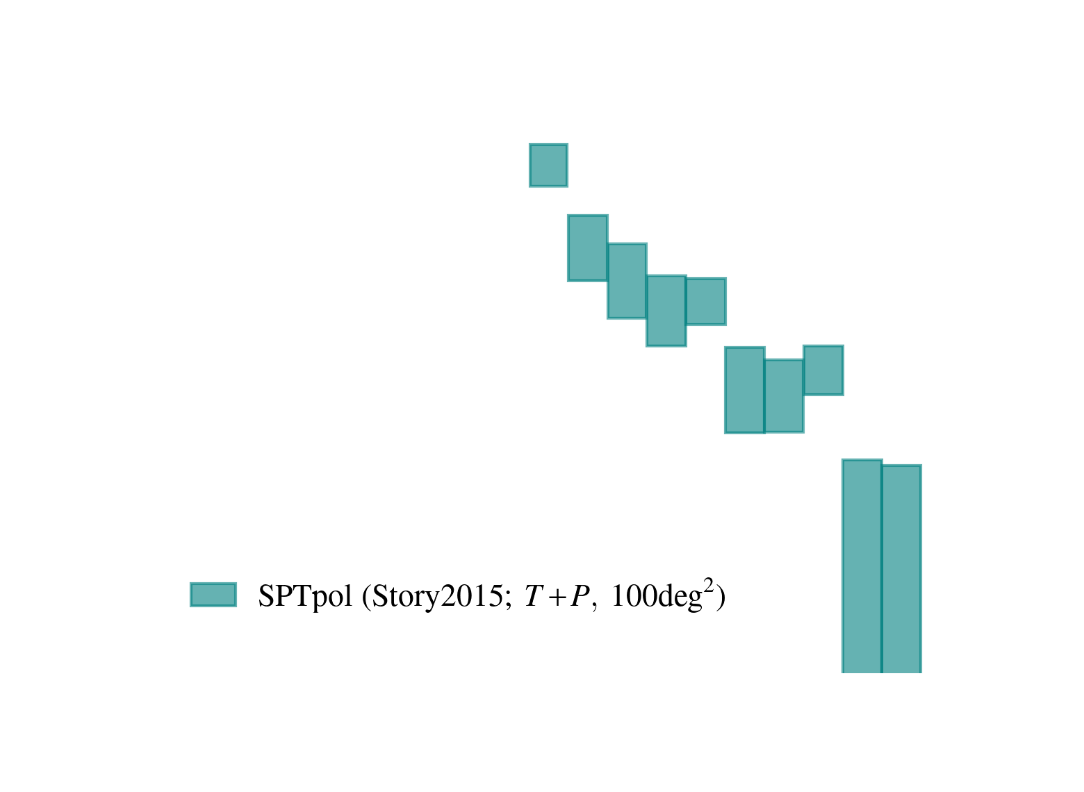
SPT-3G 2018 Imminent
SPT-3G 2019/2020 in a few months
South Pole Telescope
18
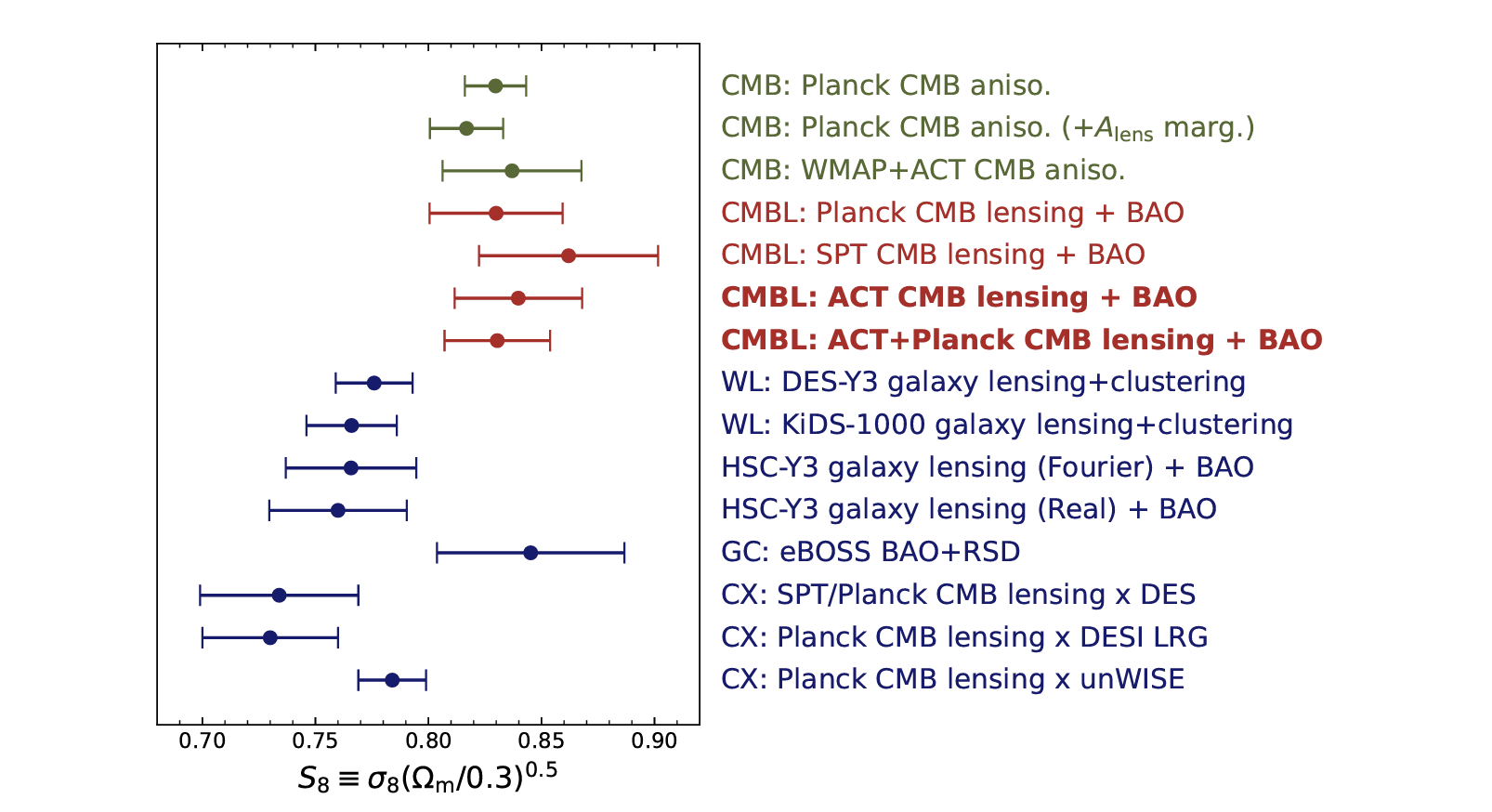
Comparison with galaxy weak lensing
19
Jeffery+ 2021
Map of from the
Dark Energy Survey
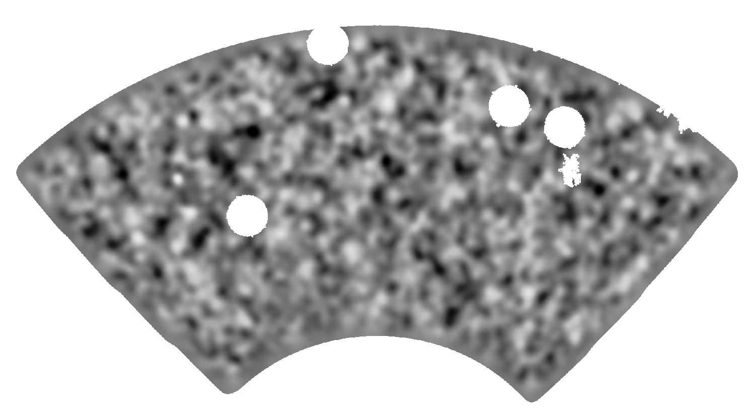
DES galaxy lensing
map (overlay)
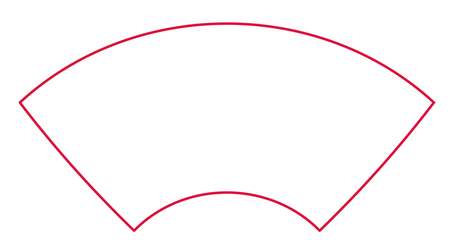
SPT-3G CMB lensing map (base)
20
(see also: Omori+2018, Chang+2023)
Comparison with galaxy weak lensing
21
Comparison with galaxy weak lensing
Qu+ 2023
Optimal lensing
22
(Millea+ 2021; see also Carron+ 2019)
CMB lensing forward modeling
+ higher
Credit: Marius Millea
Incoming data
Simons Observatory
South Pole Observatory
23
Incoming data
Simons Observatory
South Pole Observatory
23
Summary
24
- The most common approach to reconstruct a CMB lensing map: Quadratic estimator.
- Temperature maps have astrophysical foregrounds in them, and some treatment has to be made before/after lensing reconstruction (we now have various mitigation techniques).
- Polarization maps are cleaner but require low-noise surveys to produce powerful lensing maps.
- Forward modeling (optimal) approaches are becoming increasingly important as the noise levels in the polarization channel continue to decrease.
- Currently at an exciting time -- we already have good data, but the quality will become orders of magnitude better soon.